What is a Polynomial Commitment?
A commitment is a way to “lock” a message, resulting in a commitment value. This value is referred to as the commitment to the object.
$$ c = commit(x) $$
This commitment satisfies two essential properties: Hiding and Binding.
- Hiding: $c$ does not reveal any information about $x$.
- Binding: It is computationally infeasible to find some $x’ \neq x$ such that $c = commit(x’)$.
The simplest commitment mechanism is a hash function. Note that such a hash function must provide cryptographic security, such as SHA256 or Keccak. Besides hash functions, there are also schemes like Pedersen commitments.
As the name suggests, a polynomial commitment is a commitment to a polynomial. If we express a polynomial in the following form:
$$ f(X) = a_0 + a_1X + a_2X^2 + \cdots + a_nX^n $$
It can be uniquely identified by its coefficient vector:
$$ (a_0, a_1, a_2, \ldots, a_n) $$
How to Commit to a Polynomial?
First method: Hash the coefficient vector to get a unique value that binds the commitment to the polynomial.
$$ C_1 = \textrm{SHA256}(a_0 \parallel a_1 \parallel a_2 \parallel \cdots \parallel a_n) $$
For example, consider a polynomial $f(x) = 3 + 4x + 5x^2$. Its coefficient vector is $[3, 4, 5]$. Convert this vector into a string and concatenate the coefficients: "3\parallel 4\parallel 5". Then, hash this string using SHA256. Suppose the hash output is:
a1f4d3b3c6e4b7d5d6e4f5c6a7b8c9d0e1f2a3b4c5d6e7f8g9h0i1j2k3l4m5n6o7p8q9r0
This hash value uniquely represents the polynomial $f(x) = 3 + 4x + 5x^2$.
Second method: Use Pedersen commitments. Compute an elliptic curve point using a set of randomly chosen bases:
$$ C_2 = a_0 G_0 + a_1 G_1 + \cdots + a_n G_n $$
If the Prover commits to a polynomial, the Verifier can evaluate the polynomial based on the commitment and request proof of the correctness of the evaluation. Suppose $C = Commit(f(X))$. The Verifier may query the Prover for the value of the polynomial at $X = \zeta$. The Prover then provides not only the computed value (e.g., $f(\zeta) = y$) but also a proof $\pi$ to demonstrate that $C$ corresponds to a polynomial $f(X)$ whose value at $X = \zeta$ is indeed $y$.
This property of “evaluating with proof” makes polynomial commitments highly useful. It can be seen as a lightweight form of verifiable computation. That is, the Verifier delegates the computation of the polynomial $f(X)$ to a remote machine (the Prover) and verifies the correctness of the result $y$ with less computational effort than directly computing $f(X)$. Polynomial commitments can also be used to prove properties of secret data (provided by the Prover), such as satisfying a polynomial equation, without revealing the data itself.
Although this verifiable computation is limited to polynomial operations, general-purpose computation can be reduced to polynomial computation in various ways, enabling general-purpose verifiable computation based on polynomial commitments.
Using the Pedersen commitment method described above for polynomial coefficients, we can employ the Bulletproof-IPA protocol to construct evaluation proofs, resulting in another polynomial commitment scheme. Additionally, there are other schemes like KZG10, FRI, Dark, and Dory.
KZG10 Construction
Compared to the random bases used in Pedersen commitments (which are randomly generated points without internal relationships), KZG10 polynomial commitments require a set of bases with internal algebraic structure. These structured bases are derived from a random secret $\chi$, known as the structured reference string (SRS), which forms the foundation of KZG10. Here are the details:
Given the polynomial:
$$ f(X) = a_0 + a_1 X + a_2 X^2 + \dots + a_{d-1} X^{d-1} $$
where $a_0, a_1, a_2, \ldots, a_{d-1}$ are the coefficients of the polynomial.
Set $X = \chi$, and substitute into the polynomial:
$$ f(\chi) = a_0 + a_1 \chi + a_2 \chi^2 + \dots + a_{d-1} \chi^{d-1} $$
Key Notes:
- $\chi$ is a special secret random number provided by a trusted third party. It is also referred to as the trapdoor and is only used during the initialization phase (Setup) to generate system parameters. Neither the Prover nor the Verifier should know $\chi$. After the Setup phase, $\chi$ must be completely destroyed to ensure the system’s security.
Thus, the public parameters —— Structured Reference String(SRS) are:
$$ \mathsf{srs} = (G_0, G_1, G_2, \dots, G_{d-1}, H_0, H_1) $$
Where:
$$ G_0 = G,\quad G_1 = \chi G,\quad G_2 = \chi^2 G,\quad \dots,\quad G_{d-1} = \chi^{d-1} G,\quad H_0 = H,\quad H_1 = \chi H $$
Notes:
- $G$ and $H$ are the generators of elliptic curve groups $\mathbb{G}$ and $\mathbb{H}$, respectively. The powers of $\chi$ are embedded into elliptic curve points via scalar multiplication with the generators (e.g., $G_2 = \chi^2 G$ is computed by adding $G$ to itself $\chi^2$ times on the elliptic curve).
- Besides $G \in \mathbb{G}$ and $H \in \mathbb{H}$, the two groups are linked by a bilinear map $e: \mathbb{G} \times \mathbb{H} \to \mathbb{G}_T$ (where $\mathbb{G}_T$ is another elliptic curve group). Some important properties of the bilinear map are:
- Bilinearity: For all $G \in \mathbb{G}, H \in \mathbb{H}$, and integers $a, b$, $e(a \cdot G, b \cdot H) = e(G, H)^{ab}$.
- Non-degeneracy: If $G$ is a generator of $\mathbb{G}$ and $H$ is a generator of $\mathbb{H}$, then $e(G, H)$ is a generator of $\mathbb{G}_T$.
- Efficient Computability: The bilinear map $e$ can be computed in polynomial time.
Returning to the SRS:
$$ \mathsf{srs} = (G_0, G_1, G_2, \dots, G_{d-1}, H_0, H_1) $$
After initialization, these structured bases are indistinguishable from random bases from an external perspective. This achieves our goal.
Setup Phrase
The SRS is divided into two parts during Setup Phase:
- $\mathbb{G}$ Basis Vectors: $\mathsf{srs}_ {\mathbb{G}} = (G_0, G_1, G_2, \dots, G_{d-1})$ where $G_i = \chi^i G$ ( $i$ is the index, $0 \leq i < d$ ).
- $\mathbb{H}$ Basis Vectors: $\mathsf{srs}_{\mathbb{H}} = (H_0, H_1)$ where $H_i = \chi^i H$ (used for auxiliary verification, such as divisibility checks).
When using Groth’s notation:
$$ [1]_1 \triangleq G,\quad [1]_2 \triangleq H $$
The KZG10 system parameters (SRS) can be expressed as:
$$ \begin{align} \mathsf{srs} & = ({\color{Violet} [} {\color{Red} 1} {\color{Violet} ]_1} ,{\color{Violet} [} {\color{Red} \chi} {\color{Violet} ]_1} ,{\color{Violet} [} {\color{Red} \chi^2} {\color{Violet} ]_1} ,{\color{Violet} [} {\color{Red} \chi^3} {\color{Violet} ]_1} ,\ldots,{\color{Violet} [} {\color{Red} \chi^{d-1}} {\color{Violet} ]_1} ,{\color{Green} [}{\color{Brown} 1} {\color{Green} ]_2} ,{\color{Green} [} {\color{Brown} \chi} {\color{Green} ]_2} )\ & = ({\color{Red} 1} \cdot {\color{Violet} G} ,{\color{Red} \chi} {\color{Violet} G} ,{\color{Red} {\chi^2}} {\color{Violet} G} ,{\color{Red} {\chi^3}}{\color{Violet} G} ,\ldots ,{\color{Red} {\chi^{d-1}}}{\color{Violet} G} ,{\color{Brown} 1} \cdot {\color{Green} H} , {\color{Brown} \chi}{\color{Green} H}) \end{align} $$
After this Setup phase, the Prover can use the SRS to commit to a polynomial $f(X)$.
Polynomial Commitment
For a polynomial:
$$ f(X) = a_0 + a_1 X + a_2 X^2 + \dots + a_{d-1} X^{d-1} $$
The Prover commits to the coefficient vector $[a_0, a_1, a_2, \dots, a_{d-1}]$ using the $\mathbb{G}$ part of the SRS:
$$ C_{f(X)} = a_0 G_0 + a_1 G_1 + \cdots + a_{d-1} G_{d-1} $$
Substituting $G_i = \chi^i G$:
$$ C_{f(X)} = a_0 G + a_1 (\chi G) + a_2 (\chi^2 G) + \cdots + a_{d-1} (\chi^{d-1} G) $$
Factoring out $G$:
$$ C_{f(X)} = (a_0 + a_1 \chi + a_2 \chi^2 + \cdots + a_{d-1} \chi^{d-1}) G $$
This simplifies to:
$$ C_{f(X)} = f(\chi) \cdot G $$
If using Groth’s notation:
$$ C_{f(X)} = [f(\chi)]_1 $$
In summary:
-
$C_{f(X)}$, $[f(\chi)]_1$, and $f(\chi) G$ all represent the same thing: embedding the finite field element $f(\chi)$ (the evaluation of the polynomial $f(X)$ at the secret point $\chi$) into the elliptic curve group $\mathbb{G}$.
-
In $C_{f(X)} = [f(\chi)]_1$, the notation $[f(\chi)]_1$ indicates that the Prover commits to the value $f(\chi)$ at the secret point $\chi$ using the generator $[1]_1$ (i.e., $G$).
Evaluation Proofs
Next, let us construct an Open proof for $f(\zeta) = y$. The core objective is to make the verification process simpler and more efficient. The approach is to transform the direct verification of $C_{f(X)}$ into an indirect verification of $f(\zeta) = y$, which involves using $C_q$. Here are the key steps:
1. Decomposing Using the Polynomial Remainder Theorem
Based on the Polynomial Remainder Theorem (which states that if a polynomial $f(X)$ is divided by a linear polynomial $(X-\zeta)$, the remainder is $f(\zeta)$ ), we can decompose the polynomial $f(X)$ as follows:
$$ f(X) = q(X) \cdot (X-\zeta) + y $$
Where:
- $(X-\zeta)$ is a linear polynomial;
- $q(X)$ is the quotient polynomial;
- $y$ is the remainder, which is a constant;
- If $f(\zeta) \neq y$, then $g(X) = f(X) - y$ cannot be divided evenly by $(X-\zeta)$.
This equation shows that any polynomial $f(X)$ can be expressed as the product of a quotient polynomial $q(X)$ and $(X-\zeta)$, plus a remainder, which is the constant $y$.
When $X = \zeta$, $(X-\zeta) = 0$, so the term $q(X) \cdot (X-\zeta)$ becomes $0$, reducing the equation to $f(\zeta) = y$.
Let us reverse-engineer the above equation: $f(X) = q(X) \cdot (X-\zeta) + y$. Assume $f(\zeta) = y$, and construct a new polynomial $g(X)$, defined as $g(X) = f(X) - y$.
- When $X = \zeta$, $f(\zeta) = y$, so $g(X)$ evaluates to $g(\zeta) = f(\zeta) - y = 0$, meaning that $\zeta$ is a root of $g(X)$.
- If $\zeta$ is a root of $g(X)$, then $g(X)$ must be divisible by $(X-\zeta)$, which is an irreducible linear polynomial. Therefore, $g(X)$ can be expressed as $g(X) = q(X) \cdot (X-\zeta)$, where $q(X)$ is the quotient polynomial.
- Substituting $g(X)$ back into $g(X) = f(X) - y$, we get: $q(X) \cdot (X-\zeta) = f(X) - y$. Rearranging gives: $f(X) = q(X) \cdot (X-\zeta) + y$.
2. Proving $f(\zeta) = y$
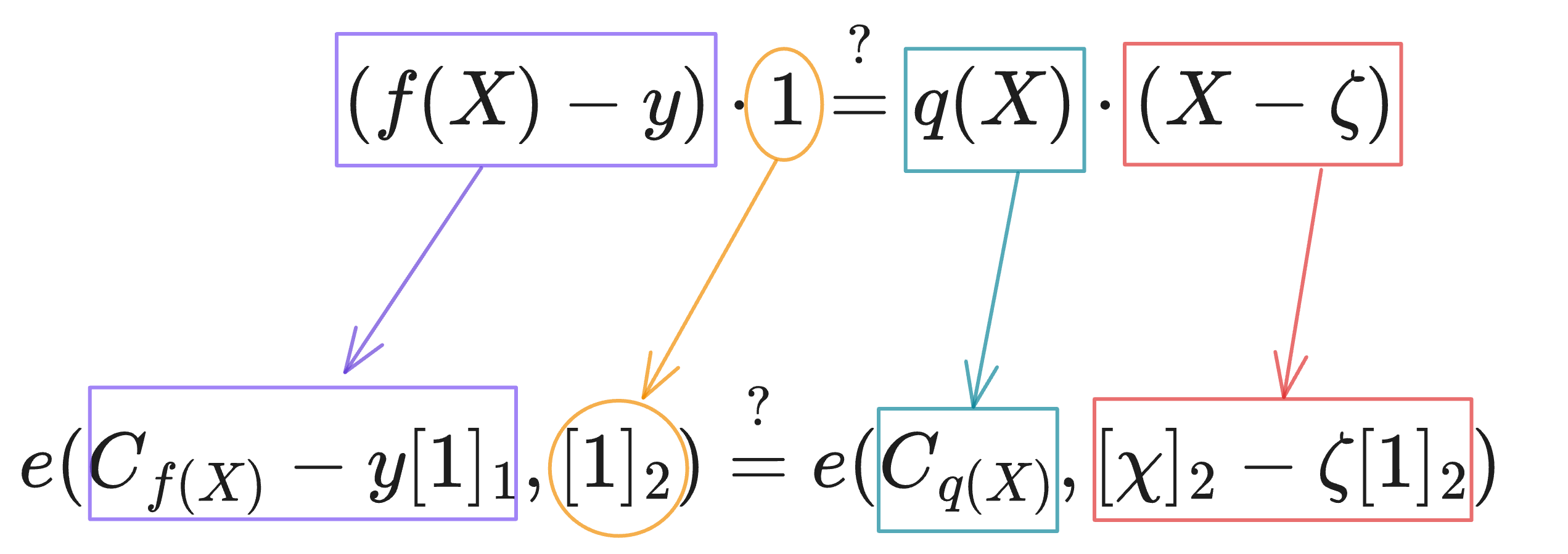
The Prover can provide a commitment to the quotient polynomial $q(X)$, denoted as $C_q$ (where $C_q$ is defined as $C_q = q(\chi) \cdot G$), as proof that $f(\zeta) = y$. The Verifier can then check whether $[q(\chi)]_1$ satisfies the divisibility condition to validate the proof. If $f(\zeta) \neq y$, then $g(X)$ cannot be divided evenly by $(X-\zeta)$, and the commitment $C_q$ provided by the Prover will fail the divisibility check:
$$ (f(X) - y) \cdot 1 \overset{?}{=} q(X) \cdot (X-\zeta) $$
Key notes:
Why Include the $\cdot 1$ in the Verification Equation?
This is because pairing (bilinear mapping) is used, specifically $e: \mathbb{G} \times \mathbb{H} \to \mathbb{G}_T$. Here:
- $\mathbb{G}$ and $\mathbb{H}$ are two groups defined over the domain;
- $\mathbb{G}_T$ is the target group of the bilinear map.
Pairing requires inputs to appear in pairs, such as $(a, b)$ or $(c, d)$, and cannot accept a single input.
Let us first examine the right-hand side of the equation. The commitment $C_q = [q(\chi)]_1$, and $(X-\zeta)$ can be expressed using the structured reference string (SRS) as $[\chi-\zeta]_1$, i.e., $(\chi-\zeta) \cdot G$. Therefore: $q(X) \cdot (X-\zeta) \quad \rightarrow \quad C_q \cdot [\chi-\zeta]_1$
As mentioned earlier, pairing requires inputs to appear in pairs. The left-hand side must also have two components. The $\cdot 1$ on the left-hand side can be seen as a placeholder. Here, $1$ corresponds to a group element on the elliptic curve, denoted as $[1]_ 1$, which is the generator $g$ of the group $\mathbb{G}$. Thus: $(f(X)-y) \cdot 1 \quad \leftrightarrow \quad C_{f(X)} - y \cdot g$
In summary:
- The $\cdot 1$ ensures that the input components and their positions are aligned, so pairing can correctly apply the bilinear map.
- The $\cdot 1$ does not affect the overall computation result.
3. Divisibility Verification Using Pairing
The commitment $C_{f(X)}$ is an element in group $\mathbb{G}$. Through the additive homomorphic property of commitments and the bilinear map $e: \mathbb{G} \times \mathbb{H} \to \mathbb{G}_T$, the Verifier can validate the divisibility condition in $\mathbb{G}_T$ as follows:
$$ e(C_{f(X)} - y[1]_ 1, [1]_ 2) \overset{?}{=} e(C_{q(X)}, [\chi]_ 2 - \zeta [1]_ 2) $$
Explanation of the Above Equation
- Left-Hand Side: $e(C_{f(X)} - y[1]_1, [1]_2)$ pairs the commitment of $f(X) - y$ with the generator of $\mathbb{H}$, producing a result in the target group $\mathbb{G}_T$.
-
This can be decomposed based on the groups involved:
- $C_{f(X)} - y[1]_1$ is in group $\mathbb{G}$.
- $[1]_2$ is the generator of group $\mathbb{H}$.
Specifically:
- $C_{f(X)}$ is the commitment to the polynomial $f(X)$: $C_{f(X)} = [f(\chi)]_1$.
- $y[1]_1$ is the commitment to the constant $y$: $y[1]_1 = y \cdot G$.
- $[1]_2$ is the generator of group $\mathbb{H}$.
-
Right-Hand Side: $e(C_{q(X)}, [\chi]_2 - \zeta [1]_2)$ pairs the commitment of the quotient polynomial $q(X)$ with the commitment of $(\chi-\zeta)$, producing a result in the target group $\mathbb{G}_T$.
-
This can also be decomposed:
- $C_{q(X)}$ is in group $\mathbb{G}$.
- $[\chi]_2 - \zeta[1]_2$ is in group $\mathbb{H}$.
Specifically:
- $C_{q(X)}$ is the commitment to $q(X)$: $C_{q(X)} = [q(\chi)]_1$.
- $[\chi]_2$ represents the secret $\chi$ in group $\mathbb{H}$: $[\chi]_2 = \chi \cdot H$.
- $\zeta[1]_2$ represents the constant $\zeta$ in group $\mathbb{H}$: $\zeta[1]_2 = \zeta \cdot H$.
-
This effectively validates the divisibility condition:
$$ f(\chi) - y \overset{?}{=} q(\chi) \cdot (\chi - \zeta) $$
4. Reducing Computation Complexity
The above verification requires the Prover to compute the division of the polynomial:
$$ q(X) = \frac{f(X) - y}{X-\zeta} $$
Polynomial division can be computationally expensive, especially when $f(X)$ is a high-degree polynomial. To reduce the computational cost, the verification equation:
$$ (f(X)-y) \cdot 1 \overset{?}{=} q(X) \cdot (X-\zeta) $$
can be transformed into:
$$ f(X) + \zeta \cdot q(X) - y = q(X) \cdot X $$
This transformation simplifies the computation in the KZG commitment verification process, aligning elliptic curve point calculations with the existing system parameters (SRS). By doing so, the Verifier avoids expensive scalar multiplications (e.g., computing $\zeta[1]_2$).
After transformation, we can further understand the role of pairing:
$$ f(X) + \zeta \cdot q(X) - y = q(X) \cdot X $$
$$ e(C_{f(X)} + \zeta \cdot C_{q(X)} - y \cdot [1]_ 1, [1]_ 2) \overset{?}{=} e(C_{q(X)}, [\chi]_ 2) $$
By analyzing the relationship between the transformed equation and the pairing-based verification process above, we can revisit and clarify some key concepts:
-
Pairing $e(\cdot, \cdot)$:
Pairing is a bilinear map defined as $e: \mathbb{G} \times \mathbb{H} \to \mathbb{G_T}$, where:- $\mathbb{G}$ and $\mathbb{H}$ are two distinct elliptic curve groups.
- $\mathbb{G_T}$ is the target group resulting from the bilinear map.
-
Commitments $C_{f(X)}$ and $C_{q(X)}$:
These are the polynomial commitments for $f(X)$ and $q(X)$, respectively. Typically, these commitments are generated using schemes like Pedersen commitments, which map polynomials to specific points on an elliptic curve. -
Left Side of the Pairing Equation:
In the pairing equation: $e(C_{f(X)} + \zeta \cdot C_{q(X)} - y \cdot [1]_ 1, [1]_ 2)$,the term $C_{f(X)} + \zeta \cdot C_{q(X)} - y \cdot [1]_ 1$ represents the commitment to the polynomial $f(X) + \zeta \cdot q(X) - y$. Meanwhile, the right-hand side $e(C_{q(X)}, [\chi]_ 2)$ corresponds to the commitment $q(X)$ paired with the structured reference string (SRS) element $[\chi]_2$.
Notes:
If you look closely at the left side of the pairing equation, you’ll notice that only $y$ is explicitly multiplied by $[1]_ 1$ (the generator of group $\mathbb{G}$ ). You might wonder why $C_{f(X)}$ and $\zeta \cdot C_{q(X)}$ do not also include $\cdot 1$. Here’s why:
- What is $y \cdot [1]_1$?
The term $y \cdot [1]_ 1$ represents the constant $y$ embedded into the elliptic curve group $\mathbb{G}$. In pairing-based proof systems, constants like $y$ cannot be directly added to other elliptic curve elements (such as $C_{f(X)}$ or $C_{q(X)}$). Before addition, the constant $y$ must first be mapped into the curve by multiplying it with the generator $[1]_1$.
- Why Don’t $C_{f(X)}$ and $\zeta \cdot C_{q(X)}$ Require This?
- $C_{f(X)}$ and $\zeta \cdot C_{q(X)}$ are already elements in the group $\mathbb{G}$ because they are commitments derived from polynomials $f(X)$ and $q(X)$. These commitments are elliptic curve points and naturally reside in the same group.
- Constants like $y$, however, are scalar values (not curve points) and need to be explicitly converted into elliptic curve elements by multiplying with $[1]_1$.
- Ensuring Compatibility:
In order to perform addition within the group $\mathbb{G}$, all terms must be in the same domain. Thus, $y$ must be multiplied by $[1]_ 1$ to become a group element, ensuring it can be added to $C_{f(X)}$ and $\zeta \cdot C_{q(X)}$.
If you understand the reasoning behind the left side of the equation, you should have no difficulty grasping the right side as well. This concludes the explanation of the pairing operation in this context!
Proof Aggregation for Open at the Same Point
In a larger security protocol, when multiple polynomial commitments are used simultaneously, their Open operations can be aggregated into a single process. This is achieved by combining multiple polynomials into a single larger polynomial, allowing batch verification of the original polynomials by opening just one point.
Suppose we have multiple polynomials, $f_1(X)$ and $f_2(X)$. The Prover wants to prove to the Verifier that $f_1(\zeta) = y_1$ and $f_2(\zeta) = y_2$. These can be expressed as:
$$ \begin{array}{l} f_1(X) = q_1(X) \cdot (X-\zeta) + y_1\ f_2(X) = q_2(X) \cdot (X-\zeta) + y_2 \end{array} $$
Using a random scalar $\nu$, the Prover can combine $f_1(X)$ and $f_2(X)$ into a single temporary polynomial $g(X)$:
$$ g(X) = f_1(X) + \nu \cdot f_2(X) $$
Then, based on the Polynomial Remainder Theorem, we can derive the following equality for verification:
$$ g(X) - (y_1 + \nu \cdot y_2) = (X - \zeta) \cdot (q_1(X) + \nu \cdot q_2(X)) $$
To understand how this equality is derived, let’s revisit the earlier concepts:
Since we know $f_1(X) = q_1(X) \cdot (X-\zeta) + y_1$, $f_2(X) = q_2(X) \cdot (X-\zeta) + y_2$, and $g(X) = f_1(X) + \nu \cdot f_2(X)$, we can substitute $f_1(X)$ and $f_2(X)$ into $g(X)$:
$$ \begin{align} g(X) &= q_1(X) \cdot (X-\zeta) + y_1 + \nu \cdot (q_2(X) \cdot (X-\zeta) + y_2)\\ g(X) &= q_1(X) \cdot (X-\zeta) + y_1 + \nu \cdot q_2(X) \cdot (X-\zeta) + \nu \cdot y_2\\ g(X) &= q_1(X) \cdot (X-\zeta) + \nu \cdot q_2(X) \cdot (X-\zeta) + y_1 + \nu \cdot y_2\\ g(X) - (y_1 + \nu \cdot y_2) &= q_1(X) \cdot (X-\zeta) + \nu \cdot q_2(X) \cdot (X-\zeta)\\ g(X) - (y_1 + \nu \cdot y_2) &= (X-\zeta) \cdot (q_1(X) + \nu \cdot q_2(X)) \end{align} $$
Here, $q_1(X) + \nu \cdot q_2(X)$ can be regarded as the “quotient polynomial,” denoted as $q(X)$. That is:
$$ q(X) = q_1(X) + \nu \cdot q_2(X) $$
Proof Aggregation Using Homomorphism
Now, suppose the proof of $f_1(X)$ at $X = \zeta$ is $\pi_1$, and the proof of $f_2(X)$ at $X = \zeta$ is $\pi_2$. By leveraging the additive homomorphism of the group, the Prover can obtain the commitment to the quotient polynomial $q(X)$:
$$ [q(\chi)]_1 = \pi = \pi_1 + \nu \cdot \pi_2 $$
Additive Homomorphism: For two groups $\mathbb{G}$ and $\mathbb{H}$, if a mapping $\phi: \mathbb{G} \to \mathbb{H}$ satisfies the condition $\forall a, b \in \mathbb{G}$, $\phi(a + b) = \phi(a) + \phi(b)$, then $\phi$ is a homomorphism. (Note: Depending on the group definition, the operation could be addition or multiplication.)
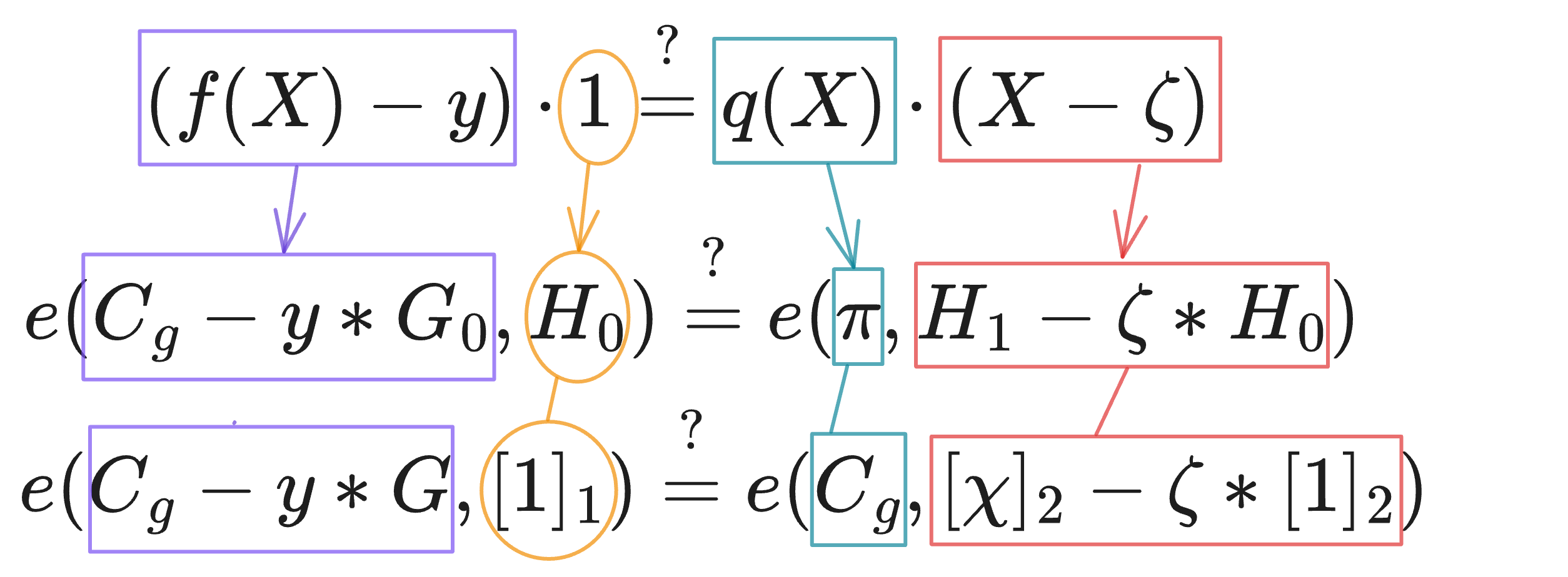
Thus, as long as the Verifier sends the Prover an additional random scalar $\nu$, both parties can fold two (or even multiple) polynomial commitments into a single commitment $C_g$:
$$ C_g = C_1 + \nu \ast C_2 $$
Why use the operator $\ast$ ? In practice, this is equivalent to $C_g = C_1 + \nu \cdot C_2$. The $\ast$ symbol is used to represent the computational implementation of the operation (e.g., a scalar multiplication function in code), rather than the mathematical scalar multiplication symbol.
The folded commitment $C_g$ can then be used to verify the evaluations of multiple polynomials at a single point:
$$ y_g = y_1 + \nu \cdot y_2 $$
Here, $y_1$ and $y_2$ are the values of the polynomials $f_1(X)$ and $f_2(X)$ at a specific point.
Through folding, multiple evaluation proofs are aggregated into one. The Verifier only needs to verify whether $C_g$ equals $y_g$ at the given point to simultaneously confirm that $f_1(X)$ and $f_2(X)$ evaluate to $y_1$ and $y_2$ at the specified point:
$$ e(C_g - y \ast G_0, H_0) \overset{?}{=} e(\pi, H_1 - \zeta \ast H_0) $$
This greatly simplifies the verification process.
Security Analysis Using Schwartz-Zippel Lemma
The Schwartz-Zippel Lemma states that for a non-zero polynomial $P(X)$ of degree $d$, the probability that $P(\nu) = 0$ for a randomly chosen $\nu$ in a finite field $\mathbb{F}_p$ is at most $\frac{d}{p}$.
From this, we derive the following:
- Higher degree increases forgery probability: If the degree $d$ of $P(X)$ is large, the probability of $P(X) = 0$ increases.
- Larger finite field decreases forgery probability: If the size of the finite field $p$ is sufficiently large, the probability of $P(X) = 0$ becomes very small.
For two different polynomials $f_1(X)$ and $f_2(X)$, if the Prover tries to forge new polynomials $f_1’(X)$ and $f_2’(X)$ such that the folded result remains the same, i.e.:
$$ f_1(X) + \nu f_2(X) = f_1’(X) + \nu f_2’(X), $$
this is equivalent to:
$$ (f_1(X) - f_1’(X)) + \nu (f_2(X) - f_2’(X)) = 0 $$
Let:
$$ \Delta_1(X) = f_1(X) - f_1’(X), \quad \Delta_2(X) = f_2(X) - f_2’(X) $$
then:
$$ \Delta_1(X) + \nu \Delta_2(X) = 0 $$
To satisfy this equation, the Prover must find a specific $\nu$, meaning $\nu$ must be a solution to the linear relationship between $\Delta_1(X)$ and $\Delta_2(X)$. If $\Delta_1(X)$ and $\Delta_2(X)$ are non-zero polynomials, their degree is:
$$ \max(\deg(\Delta_1), \deg(\Delta_2)), $$
and the probability of $\Delta_1(X) + \nu \cdot \Delta_2(X) = 0$ is at most:
$$ \frac{\max(\deg(\Delta_1), \deg(\Delta_2))}{p} $$
-
Low-degree case:
Suppose $\deg(\Delta_1) = 2$ and $\deg(\Delta_2) = 3$, then $\max(\deg(\Delta_1), \deg(\Delta_2)) = 3$. For a finite field of size $p = 2^{256}$, the forgery probability is: $\frac{3}{2^{256}}$This is an extremely small probability, making forgery nearly impossible.
-
High-degree case:
Suppose $\deg(\Delta_1) = 100$ and $\deg(\Delta_2) = 200$, then $\max(\deg(\Delta_1), \deg(\Delta_2)) = 200$. For a finite field of size $p = 2^{256}$, the forgery probability is: $\frac{200}{2^{256}}$.While the probability increases slightly, it is still negligible.
Conclusion
The probability of a randomly chosen $\nu$ leading to a successful forgery is extremely small, effectively zero. Moreover, introducing the random scalar $\nu$ only involves a linear combination of existing commitments, which does not leak any information about the secret $\chi$.
Instead, $\nu$ ensures the uniqueness of the random linear combination, preventing the Prover from forging polynomials. As a result, the aggregation of polynomials does not compromise the binding property of the commitments, as guaranteed by the Schwartz-Zippel Lemma.
Protocol:
Public Inputs:
- $C_{f_1} = [f_1(\chi)]_ 1$, $C_{f_2} = [f_2(\chi)]_ 1$, $\zeta$, $y_1$, $y_2$
Private Inputs:
- $f_1(X)$, $f_2(X)$
Proof Goal:
Prove that $f_1(\zeta) = y_1$ and $f_2(\zeta) = y_2$
Protocol Steps:
Step 1: Verifier issues a challenge scalar $\nu$.
Step 2: Prover computes $q(X) = q_1(X) + \nu \cdot q_2(X)$ and sends $\pi = [q(\chi)]_1$ to the Verifier.
Step 3: Verifier computes $C_g = C_{f_1} + \nu \cdot C_{f_2}$ and $y_g = y_1 + \nu \cdot y_2$, then verifies the following pairing equation:
$$ e(C_g - [y_g]_1, [1]_2) \overset{?}{=} e(\pi, [\chi-\zeta]_2) $$
Let’s demonstrate the execution of this protocol with the following specific values:
Private Inputs(known only to the Prover):
- $f_1(X) = 3X + 1$
- $f_2(X) = 5X + 6$
Public Inputs:
- $C_{f_1} = [f_1(\chi)]_1 = [3]_1$ (commitment to $f_1(\chi)$ )
- $C_{f_2} = [f_2(\chi)]_1 = [5]_1$ (commitment to $f_2(\chi)$ )
- $\zeta = 2$ (evaluation point)
- $y_1 = f_1(\zeta) = 7$ (value of $f_1$ at $\zeta$)
- $y_2 = f_2(\zeta) = 16$ (value of $f_2$ at $\zeta$)
Proof Goal: Prove that $f_1(\zeta) = y_1$ and $f_2(\zeta) = y_2$.
(1) Step 1: Verifier issues a challenge scalar $\nu$. Assume that $\nu = 4$.
(2) Step 2: Prover computes $q(X)$ and sends $\pi = [q(\chi)]_1$.
-
Compute $q_1(X)$ and $q_2(X)$:
-
For $q_1(X)$:
$q_1(X) = \frac{f_1(X) - y_1}{X - \zeta}$, Substitute $f_1(X) = 3X + 1$ and $y_1 = 7$: $q_1(X) = \frac{(3X + 1) - 7}{X - 2} = \frac{3X - 6}{X - 2} = 3$ -
For $q_2(X)$:
$q_2(X) = \frac{f_2(X) - y_2}{X - \zeta}$, Substitute $f_2(X) = 5X + 6$ and $y_2 = 16$: $q_2(X) = \frac{(5X + 6) - 16}{X - 2} = \frac{5X - 10}{X - 2} = 5$
-
-
Combine $q_1(X)$ and $q_2(X)$ using $\nu$:
Compute $q(X) = q_1(X) + \nu \cdot q_2(X)$: $q(X) = 3 + 4 \cdot 5 = 3 + 20 = 23$
-
Compute $\pi$:
Since $q(X)$ is constant ($q(X) = 23$), $\pi = [q(\chi)]_1 = [23]_1$, Prover sends $\pi = [23]_1$ to the Verifier.
(3) Step 3: Verifier performs the verification.
The Verifier checks the pairing equation: $e(C_g - [y_g]_1, [1]_2) \overset{?}{=} e(\pi, [\chi-\zeta]_2)$
-
Compute $C_g$ (commitment to the combined polynomial) and $y_g$ (combined evaluation value):
-
$C_g = C_{f_1} + \nu \cdot C_{f_2}$:
Substitute $C_{f_1} = [3]_ 1$, $C_{f_2} = [5]_ 1$, and $\nu = 4$: $C_g = [3]_1 + 4 \cdot [5]_1 = [3 + 20]_1 = [23]_1$. -
$y_g = y_1 + \nu \cdot y_2$:
Substitute $y_1 = 7$, $y_2 = 16$, and $\nu = 4$: $y_g = 7 + 4 \cdot 16 = 7 + 64 = 71$.
-
-
Verify the left-hand pairing:
Compute $C_g - [y_g]_1$:
Substitute $C_g = [23]_1$ and $[y_g]_1 = [71]_1$: $C_g - [y_g]_1 = [23]_1 - [71]_1 = [-48]_1$Pair with $[1]_2$: $e(C_g - [y_g]_1, [1]_2) = e([-48]_1, [1]_2)$
-
Verify the right-hand pairing:
Compute $e(\pi, [\chi - \zeta]_2)$:
Substitute $\pi = [23]_1$ and $\chi - \zeta = \chi - 2$: $e(\pi, [\chi - \zeta]_2) = e([23]_1, [\chi - 2]_2)$ -
Check if both pairings are equal:
If: $e([-48]_1, [1]_2) = e([23]_1, [\chi - 2]_2)$,
then the proof is valid, confirming that $f_1(\zeta) = y_1$ and $f_2(\zeta) = y_2$.
Notes:
In the above explanation, there are some important distinctions in terminology:
- $q(\chi)$: Represents the evaluation proof.
- KZG Commitment of $q(X)$: Refers to $[q(\chi)]_1$, which is the commitment to the polynomial $q(X)$.
Polynomial Constraints and Linearization
Assume that $[f(\chi)]_1$, $[g(\chi)]_1$, and $[h(\chi)]_1$ are the KZG10 commitments of the polynomials $f(X)$, $g(X)$, and $h(X)$, respectively. If the Verifier wants to verify the following polynomial constraint:
$$ f(X) + g(X) \overset{?}{=} h(X) $$
the Verifier simply adds the commitments of the first two polynomials and checks whether the result equals $[h(\chi)]_1$:
$$ [f(\chi)]_1 + [g(\chi)]_1 \overset{?}{=} [h(\chi)]_1 $$
If the polynomial relation involves multiplication, such as:
$$ f(X) \cdot g(X) \overset{?}{=} h(X) $$
The most direct approach is to utilize the properties of bilinear groups and verify the multiplicative relationship in $\mathbb{G}_T$ by checking the following equation:
$$ e([f(\chi)]_1, [g(\chi)]_2) \overset{?}{=} e([h(\chi)]_1, [1]_2) $$
Do you fully understand the above equation? Let’s emphasize its underlying rules: The pairing $e: (\mathbb{G}, \mathbb{H}) \to \mathbb{G}_T$ implies that:
- $[f(\chi)]$ must be in group $\mathbb{G}$, denoted as $[f(\chi)]_1$;
- $[g(\chi)]$ must be in group $\mathbb{H}$, denoted as $[g(\chi)]_2$.
The result of $e([f(\chi)]_1, [g(\chi)]_2)$ will always lie in group $\mathbb{G}_T$.
However, if the Verifier only has the commitment $[g(\chi)]_1$ in group $\mathbb{G}$ (instead of $[g(\chi)]_2$ in group $\mathbb{H}$), then the Verifier cannot use the bilinear pairing operation to verify the multiplication constraint.
An alternative method is to open all three polynomials at the same challenge point $X = \zeta$ and verify whether the opened values satisfy the multiplication constraint. Suppose the Verifier wants to verify:
$$ f(X) \cdot g(X) \overset{?}{=} h(X). $$
- The Prover sends the values $f(\zeta)$, $g(\zeta)$, and $h(\zeta)$.
- The Prover provides three evaluation proofs $\pi_{f(\zeta)}$, $\pi_{g(\zeta)}$, and $\pi_{h(\zeta)}$, proving that these values match their respective commitments.
The Verifier then:
- Checks whether $f(\zeta) \cdot g(\zeta) \overset{?}{=} h(\zeta)$.
- Verifies the correctness of the three evaluation proofs.
This approach allows the verification of more complex polynomial constraints, such as:
$$ f_1(X)f_2(X) + h_1(X)h_2(X)h_3(X) + g(X) = 0 $$
Suppose the Verifier already has the KZG10 commitments of these polynomials: $[f_1(\chi)]_1$, $[f_2(\chi)]_1$, $[h_1(\chi)]_1$, $[h_2(\chi)]_1$, $[h_3(\chi)]_1$, and $[g(\chi)]_1$. The most straightforward approach is for the Prover to open these six commitments at the challenge point $X = \zeta$, sending the six values and their corresponding evaluation proofs:
$$ (f_1(\zeta), \pi_{f_1}), (f_2(\zeta), \pi_{f_2}), (h_1(\zeta), \pi_{h_1}), (h_2(\zeta), \pi_{h_2}), (h_3(\zeta), \pi_{h_3}), (g(\zeta), \pi_{g}) $$
The Verifier:
- Verifies the six evaluation proofs.
- Checks whether:
$$ f_1(\zeta)f_2(\zeta) + h_1(\zeta)h_2(\zeta)h_3(\zeta) + g(\zeta) \overset{?}{=} 0 $$
Optimizing the Verification Process
If many polynomials are involved, the Prover must send multiple evaluation values and proofs, leading to high communication and computation costs. Is there a way to optimize this? Yes!
To reduce the number of opened polynomials, the Prover can introduce an auxiliary polynomial. Additionally, by leveraging the additive homomorphism of KZG10 commitments, the Verifier can validate complex multiplication relations without increasing communication costs.
Optimized Protocol
Step 1: Define an Auxiliary Polynomial
Define an auxiliary polynomial:
$$ L(X) = \bar{f} \cdot g(X) - h(X), $$
where $\bar{f} = f(\zeta) = c$ is the specific value of $f(X)$ at $X = \zeta$. If $f(X) \cdot g(X) = h(X)$ holds, then at $X = \zeta$, we have:
$$ L(\zeta) = c \cdot g(\zeta) - h(\zeta) = \bar{f} \cdot g(\zeta) - h(\zeta) = 0. $$
Step 2: Prover’s Operations
-
Open $f(X)$ at $X = \zeta$:
- The Prover sends $\bar{f} = f(\zeta)$ and the corresponding evaluation proof $\pi_{f(\zeta)}$ to the Verifier.
-
Construct the Commitment for $L(X)$:
- Compute $[L(\chi)]_1 = \bar{f} \cdot [g(\chi)]_1 - [h(\chi)]_1$.
- The Prover does not need to send this commitment to the Verifier, as the Verifier can construct it directly using the additive homomorphism of KZG10 commitments after receiving $\bar{f}$.
-
Open $L(X)$ at $X = \zeta$:
- The Prover proves that $L(\zeta) = 0$ by providing an evaluation proof $\pi_{L(\zeta)}$.
Step 3: Verifier’s Operations
-
Verify the evaluation proof for $f(\zeta)$:
$e([f(\chi)]_ 1 - \bar{f} \cdot [1]_ 1, [1]_ 2) \overset{?}{=} e(\pi_{f(\zeta)}, [\chi - \zeta]_ 2)$
-
Verify that $L(X)$ evaluates to zero:
$e([L(\chi)]_ 1, [1]_ 2) \overset{?}{=} e(\pi_{L(\zeta)}, [\chi - \zeta]_ 2)$
If the verification passes, this implies that $f(X) \cdot g(X) = h(X)$.
Advantages of the Optimized Protocol
Originally, the Prover needed to open three polynomials ($f(X)$, $g(X)$, and $h(X)$ ). With this optimization, only two openings are required:
- The first opening is $\bar{f}$, which provides the value $f(\zeta)$ to ensure accurate subsequent calculations.
- The second opening is $L(X)$, with the value $L(\zeta) = 0$, which indirectly verifies the multiplication constraint.
Extending to Multiple Polynomial Constraints
We can further optimize the protocol for verifying constraints involving multiple polynomials, such as:
$$ f_1(X)f_2(X) + h_1(X)h_2(X)h_3(X) + g(X) = 0 $$
Using aggregation techniques and leveraging the homomorphic properties of KZG10 commitments, the Prover can combine the constraints into a single polynomial using a random challenge scalar $\nu$. This allows the Verifier to validate complex constraints with minimal communication overhead.
Protocol:
Public Inputs: $C_{f_1} = [f_1(\chi)]_ 1$, $C_{f_2} = [f_2(\chi)]_ 1$, $C_{h_1} = [h_1(\chi)]_ 1$, $C_{h_2} = [h_2(\chi)]_ 1$, $C_{h_3} = [h_3(\chi)]_ 1$, $C_g = [g(\chi)]_ 1$
Private Inputs: $f_1(X)$, $f_2(X)$, $h_1(X)$, $h_2(X)$, $h_3(X)$, $g(X)$
Proof Goal: To prove: $f_1(X)f_2(X) + h_1(X)h_2(X)h_3(X) + g(X) = 0$
Step 1: Verifier sends $X = \zeta$
Step 2: Prover computes and sends three Openings:
$\bar{f}_1 = f_1(\zeta)$, $\bar{h}_1 = h_1(\zeta)$, $\bar{h}_2 = h_2(\zeta)$
Why does the Prover choose to send $\bar{f}_1 = f_1(\zeta)$, $\bar{h}_1 = h_1(\zeta)$, and $\bar{h}_2 = h_2(\zeta)$ instead of other values?
$h_1(X)h_2(X)h_3(X)$ is a product term. Knowing two of the values (e.g., $\bar{h}_1$ and $\bar{h}_2$) is sufficient for the Verifier to deduce $\bar{h}_3$ using the equation:
$$\bar{h}_3 = \frac{\text{known product value}}{h_1 \cdot h_2}$$
Can other values (e.g., $\bar{h}_3$) be sent instead?
Yes, sending any two values (e.g., $\bar{h}_1$ and $\bar{h}_3$) is equivalent. However, choosing different values may complicate the Verifier’s verification logic and make the process less efficient. For example, if the Prover sends $\bar{f}_1$, $\bar{h}_2$, and $\bar{h}_3$, while verification is still possible, it would involve:
- Increased verification complexity: The Verifier would need to deduce $\bar{h}_1$ from $\bar{h}_2$ and $\bar{h}_3$, making the process less intuitive.
- Potential redundant communication: If $\bar{h}_1$ is not sent, the Verifier might need to reconstruct it, adding extra computation and verification steps to the protocol.
Conclusion: Choose the simplest approach.
Step 3: Verifier sends a random scalar $\nu$.
Step 4:
Prover folds the commitments $(L(X), f_1(X), h_1(X), h_2(X))$, computes $L(X)$ and the quotient polynomial $q(X)$, and sends the commitment $[q(\chi)]_1$ as the proof of the folded polynomial evaluation at $X = \zeta$.
$$ L(X) = \bar{f}_1 \cdot f_2(X) + \bar{h}_1\bar{h}_2 \cdot h_3(X) + g(X) $$
Explanation of $L(X)$:
- $\bar{f}_1 = f_1(\zeta)$, $\bar{h}_1 = h_1(\zeta)$, and $\bar{h}_2 = h_2(\zeta)$ are the Opening values sent by the Prover in Step 2.
- $L(X)$ serves to split the proof goal into two parts:
- Fixed values $\bar{f}_1$, $\bar{h}_1$, $\bar{h}_2$ (already provided by the Prover and directly usable by the Verifier).
- Remaining polynomial components $f_2(X)$, $h_3(X)$, and $g(X)$, unified under $L(X)$.
$$ \begin{align} q(X) & = \frac{F(X)}{X-\zeta} \ & = \frac{L(X) + \nu \cdot (f_1(X) - \bar{f}_1) + \nu^2 \cdot (h_1(X) - \bar{h}_1) + \nu^3 \cdot (h_2(X) - \bar{h}_2)}{X-\zeta} \end{align} $$
How to understand the above equation for $q(X)$?
- From previous discussions, the quotient polynomial $q(X)$ is defined as:
$$q(X) = \frac{f(X) - y}{X-\zeta}$$
Here, $f(X) - y$ is a polynomial that evaluates to $0$ at $X = \zeta$ (since $f(\zeta) = y$). Consequently, $f(X) - y$ is divisible by $X-\zeta$, and the quotient is $q(X)$.- Our proof goal is $f_1(X)f_2(X) + h_1(X)h_2(X)h_3(X) + g(X) = 0$. To verify this, we introduce the auxiliary polynomial $L(X)$.
- To reduce communication overhead, the protocol uses a folding technique. The Verifier applies a random challenge scalar $\nu$ to linearly combine multiple polynomials $(L(X), f_1(X), h_1(X), h_2(X))$ into a single polynomial: $F(X) = L(X) + \nu \cdot (f_1(X) - \bar{f}_1) + \nu^2 \cdot (h_1(X) - \bar{h}_1) + \nu^3 \cdot (h_2(X) - \bar{h}_2)$. This $F(X)$ contains all the polynomial information related to the proof goal. Since $F(X)$ is divisible by $(X-\zeta)$, the quotient is $q(X)$.
Step 5: Verifier computes the commitment to the auxiliary polynomial $L(X)$:
$$ [L(X)]_1 = \bar{f}_1 \cdot [f_2(\chi)]_1 + \bar{h}_1\bar{h}_2 \cdot [h_3(\chi)]_1 + [g(\chi)]_1 $$
The Verifier then computes the commitment to the folded polynomial:
$$ [F(X)]_1 = [L(X)]_1 + \nu \cdot [f_1(\chi)]_1 + \nu^2 \cdot [h_1(\chi)]_1 + \nu^3 \cdot [h_2(\chi)]_1 $$
Does the equation for $[F(X)]_1$ seem strange?
Why does the formula for the commitment of the folded polynomial $[F(X)]_1$ differ from the right-hand side of $F(X)$?

Can $F(X)$ be written as $F(X) = L(X) + \nu \cdot f_1(X) + \nu^2 \cdot h_1(X) + \nu^3 \cdot h_2(X)$?
Yes, we can reverse-engineer this representation:
According to the Polynomial Remainder Theorem, if a polynomial $F(X)$ is divided by a linear polynomial $(X-\zeta)$, the remainder is $F(\zeta)$. Rearranging gives: $q(X) = \frac{F(X) - F(\zeta)}{X-\zeta}$.
Since the Verifier’s validation depends on $q(X)$, the quotient polynomial $q(X)$ already enforces the correctness of the Opening values. Thus, an alternative representation of $F(X)$ and $q(X)$ is: $F(X) = L(X) + \nu \cdot f_1(X) + \nu^2 \cdot h_1(X) + \nu^3 \cdot h_2(X)$, $q(X) = \frac{F(X) - F(\zeta)}{X - \zeta}$.
The Verifier computes the evaluation of the folded polynomial at $X = \zeta$:
$$ E \overset{?}{=} F(\zeta) = \nu \cdot \bar{f}_1 + \nu^2 \cdot \bar{h}_1 + \nu^3 \cdot \bar{h}_2 $$
Here, $E$ is a concrete value computed by the Verifier, used to validate the correctness of $F(\zeta)$.
The Verifier checks the following pairing equation:
$$ e([F(X)]_1 - [E]_1 + \zeta [q(\chi)]_1, [1]_2) \overset{?}{=} e([q(\chi)]_1, [\chi]_2) $$
Optimized Protocol Summary
Using this optimized protocol, the Prover only needs to send three Openings and one evaluation proof, compared to the original approach requiring six Openings and six evaluation proofs. This greatly reduces communication overhead (i.e., proof size).